Research & Context
Tropical cyclones are a type of natural disaster that bring high winds, torrential rain, and storm surges. A tropical cyclone is defined as "[a] warm-core non-frontal synoptic-scale cyclone, originating over tropical or subtropical waters, with organized deep convection and a closed surface wind circulation about a well-defined center" (WMO 2022). The most compelling feature of a cyclone is its eye at the center which is surrounded by the eyewall, an area of extremely heavy rain and strong winds that is within 100 kilometers of the eye (Carstens et al., 2025). Beyond the eyewall, precipitation occurs in spiraling rainbands, curved bands of clouds and storms that trail away from the eye in a spiral pattern (Carstens et al., 2025). The goal of this project is to model the shape of the spiral rainbands using a polar equation.
This type of model is used by atmospheric scientists and remote sensing researchers to understand cyclone patterns and storm intensity. Yurchak (2024) found that a spiral model of cyclones correlates with maximum wind speed at a rate of 0.95, meaning the shape of the spiral is strongly related to how powerful the storm is. These models can be used in storm risk assessment to predict potential damage from cyclone winds and rains (Yi et al., 2022).
A radial (polar) framework is appropriate because tropical cyclones are fundamentally rotating systems centered around a single point, the eye. The winds of a tropical cyclone are composed of two components: tangential, which are spinning, and radial, which are inward and outward (Carstens et al., 2025). The two variables used in a polar equation, r (radius) and θ (angle), show these two types of winds directly by representing the distance from the center and the angle around the center. Yurchak (2024) explicitly fitted tropical cyclones to a logarithmic spiral using satellite images of hurricane rainbands, confirming that a spiral structure, which is much easier to model with a polar equation, is a key geometric feature of tropical cyclones.
Polar Model
Cyclones can be modeled using the polar equation , where:
- r is the distance from the cyclone's eye in km
- θ is the angle around the storm in radians
- a is the starting distance in km
- and b is the spiral tightness factor (unitless), usually 0.1 to 0.3
This equation is reasonable because the spiral rainbands of cyclones closely follow logarithmic spirals when viewed from above. Satellite radar images fit cyclone spiral signatures using a hyperbolic-logarithmic spiral, a more complex two-dimensional spiral that combines hyperbolic and logarithmic components (Yurchak, 2024). For the purposes of this project, which models cyclones from a bird's eye view, the simpler two-dimensional logarithmic spiral serves as an appropriate approximation.
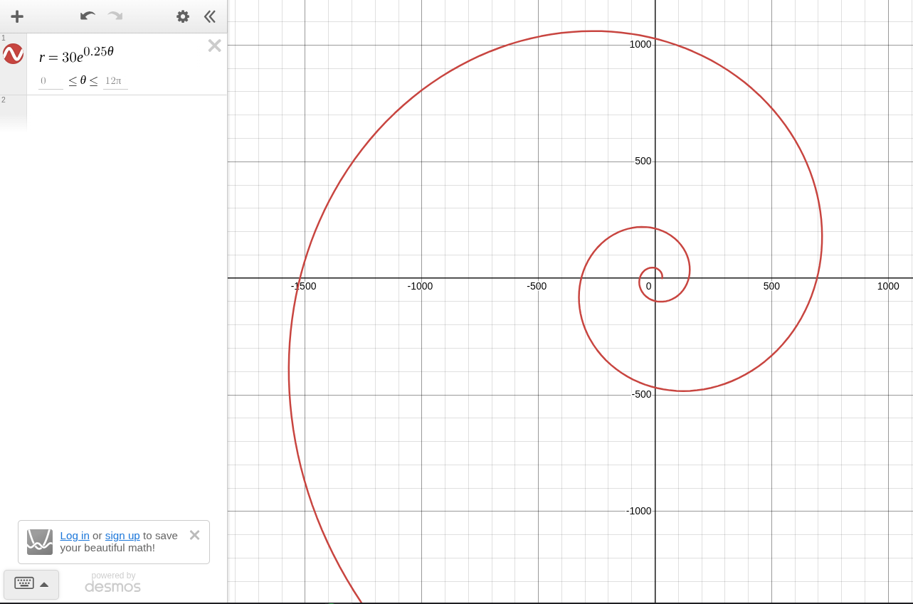
The polar equation graphed using Desmos with example values for parameters.
Calculus Based Analysis
Given , the derivative of r with respect to θ is:
This means, so long as the radius is positive and increases, the angle will increase. The rate of increase is proportional to the current radius, creating the expanding spiral shape seen in satellite imagery.
Additionally, the arc length is:
The arc length is the total length of the spiral rainband from the starting point to the outer edge of the storm.
The area enclosed by the cyclone would be:
This is the area enclosed by the equation representing the physical area the storm covers.
Example with Real Numbers
km, , ,
Therefore,
Because the derivative is always positive, so long as θ increases, the radius will increase. This leads to the equation's characteristic expanding spiral shape. As the spiral expands outward, it expands faster and faster; its angular velocity increases.
Additionally,
This means that after just two rotations, the rainband stretches over 2738 km.
Finally,
This means that after two rotations, the cyclone sweeps over an area of over 481,000 square kilometers. This area represents the total region covered by the rainband.
Cartesian Comparison
To compare to the Cartesian coordinate system, recall the following formulas:
Given the equation , and . Attempting to convert from polar to Cartesian, x and y are parametric equations. Attempting to write x as a function of y is extremely difficult, as it is difficult to isolate θ. Solving for θ in terms of y requires solving the equation , which has no algebraic solution. Furthermore, because the spiral crosses any given horizontal line multiple times, x is not a single valued function of y.
Eliminating θ leads to which mixes exponentials and inverse trig functions. Attempting to isolate y on one side of the equation would result in the parameters a and b becoming buried inside exponentials. The polar equation has several advantages. r easily gives the distance from the eye, and θ easily gives the direction from the eye. The polar equation shows immediately that the radius grows exponentially with the angle, the parameter b directly controls how quickly the spiral expands, and the parameter a directly gives the radius when θ = 1.
Though certain information is more obvious or easy to calculate in polar form, Cartesian coordinates may still be useful in real life situations when weather maps use latitude and longitude, combining cyclone information with other geographic information, and making sure data is compatible with already existing weather models and datasets that use Cartesian coordinates.
Conclusion
Tropical cyclones follow a logarithmic spiral, a shape that expands outwards at a rate proportional to its current radius. The equation captures this relationship because as the angle θ increases, the distance from the eye, r, grows exponentially. This matches satellite observations, where logarithmic spirals fit actual hurricane rainbands (Yurchak, 2024).
The derivative reveals that the rate at which the spiral expands is proportional to its current radius. The farther from the eye the storm travels, the faster the spiral itself expands. This explains why satellite images show tight curves near the eye, but broader spread out curves at the storms' edges.
The arc length represents the actual length of the spiral rainband from its starting point near the eyewall to the edge of the storm. This number is significant because it quantifies the total extent of cloud cover and precipitation that is associated with a single rainband.
Polar coordinates fit this model better than Cartesian coordinates for several reasons. A polar equation naturally shows the eye of the storm at the origin while also clearly showing the distance and position of the storm from the eye. Attempting to convert the polar equation to Cartesian yields the implicit equation that is messy and difficult to work with.
While the model shows the overall spiral shape of tropical cyclones it has multiple limitations. The model assumes that the spiral is perfectly symmetric around the eye while real cyclones have asymmetries. The model also describes shape, but not motion over time when real rainbands vary with time. Additionally, the spiral tightness determined by the parameter b is constant, when in reality b would vary with radius and angle. Finally, the model is two-dimensional and assumes a fixed center, whereas real cyclones are three dimensional and their eyes move over time.
Despite these simplifications, the logarithmic spiral model provides a powerful and clean way to describe the shape of hurricane rainbands. It demonstrates that polar coordinates are a natural model for rotating systems like tropical cyclones. As climate change continues to warm ocean waters and intensify cyclone winds and rains (Carstens et al., 2025), understanding their structure through mathematical models is important for forecasting and disaster preparation.
Works Cited
Carstens, J. D., Uejio, C. K., Powell, E., Jung, J., & Zonka, S. (2025). Tropical cyclones and climate change: An overview for the public health community. Environmental Research, 285, 122149. https://doi.org/10.1016/j.envres.2025.122149
WMO. (2022, December 16). Tropical cyclone. World Meteorological Organization. https://wmo.int/topics/tropical-cyclone
Yurchak, B. S. (2024). Estimating the intensity of tropical cyclones from spiral signatures acquired by spaceborne SAR. Remote Sensing, 16(10), 1750. https://doi.org/10.3390/rs16101750
Yi, L., Chen Peiyan, Hui, Y., Fang Pingzhi, Ting, G., Wang Xiaodong, & Shengnan, S. (2022). Parameterized tropical cyclone precipitation model for catastrophe risk assessment in China. Journal of Applied Meteorology and Climatology, 61(9), 1291-1303. https://doi.org/10.1175/jamc-d-21-0157.1